05. Distributions of Returns and Prices
Distributions of Returns and Prices
Investors are always interested in the potential appreciation or depreciation of financial assets. They'd like to be able to predict what will happen to assets in the future, hence, they'd like to be able to build models of stock prices and returns. An important first step is to think of these prices and returns as random variables , i.e. outcomes of random phenomena, that take on values as described by distributions . Distributions allow us to summarize the behavior of random variables. So, what are the distributions of returns and prices?
One strategy for getting a sense of potential future behavior is to look to the past. Let's look at some data from the stock of a familiar company with a storied past, Apple Inc.
Returns and the Historical Record
Let's look at the adjusted closing price of Apple stock (AAPL) from 1980 up until the present.

If we calculate returns and log returns on these data and plot them, we'll see something like the graphs below.

These plot look almost the same—that's because the returns and log returns for these daily data have very similar values . This is because daily returns are small—the values are close to 0, so the property \ln(1 + r) \approx r applies. But we're interested in the distribution of these values, so let's look at a histogram.
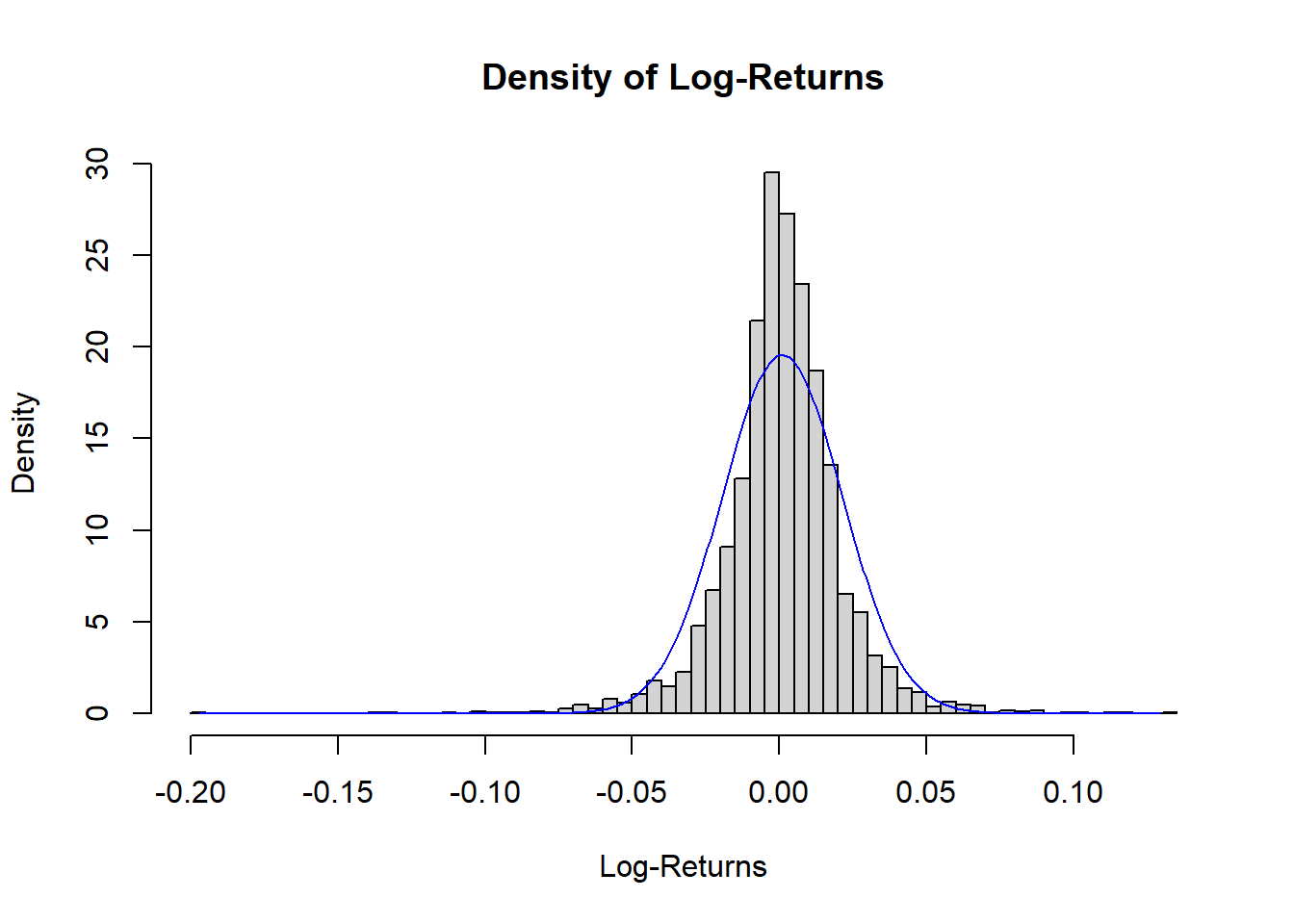
Here we've plotted a histogram of AAPL's log returns from 1980 to the present, and we've overlaid a scaled normal distribution. We can see a few things right away from this plot. First, the values are centered around 0, and in fact look roughly normal. However, the tails of the histogram clearly lie above the tails of the normal distribution. We call these "fat tails".
In general, the normal distribution can be a reasonable approximation for short-term returns and log returns for some applications. However, many analyses have shown that the data do not conform perfectly to a normal distribution, and often deviate significantly in the tails. The significance of this is that the normal distribution predicts fewer extreme events than are actually observed. The conversation about the best model for the distribution of returns has been going on for at least the past century. The best model will depend on exactly what your analysis seeks to achieve.
Normality and Long-Term Investments
Based on historical data, it may be reasonable to consider short-term returns as approximately normally distributed for some purposes. However, even if short-term returns are normally distributed, long-term returns cannot be. If r_1 = \frac{p_1 - p_0}{p_0} and r_2 = \frac{p_2 - p_1}{p_1} are normally distributed, the sum of these, r_1 + r_2 would be normally distributed. But the two-period return is not the sum of the one-period returns.
Two-period return = \frac{p_2 - p_0}{p_0}
\frac{p_2 - p_0}{p_0} + 1 = \frac{p_2 - p_0}{p_0} + \frac{p_0}{p_0} = \frac{p_2}{p_0}
= \frac{p_1}{p_0}\times\frac{p_2}{p_1}
= (1 + r_1)(1 + r_2)
The product (1 + r_1)(1 + r_2) is not normal, and becomes noticeably less normal as the product grows over time.
Take a look at the workspace below to get a feeling for how this occurs.
Workspace
This section contains either a workspace (it can be a Jupyter Notebook workspace or an online code editor work space, etc.) and it cannot be automatically downloaded to be generated here. Please access the classroom with your account and manually download the workspace to your local machine. Note that for some courses, Udacity upload the workspace files onto https://github.com/udacity , so you may be able to download them there.
Workspace Information:
- Default file path:
- Workspace type: jupyter
- Opened files (when workspace is loaded): n/a
M1L5 06 Distribution Of Stock Prices Part 2 V1
Distribution of Log Returns
So long-term prices and cumulative returns can be modeled as approximately lognormally distributed because they are products of independently, identically distributed (IID) random variables. On the other hand, log returns sum over time. Therefore, if R_1 = \ln\left(\frac{p_1}{p_0}\right) and R_2 = \ln\left(\frac{p_2}{p_1}\right) are normal, their sum, the two-period log return, is also normal. Even if they are not normal, as long as they are IID, their long-term sum will be approximately normal, thanks to the Central Limit Theorem. This is one reason why using log returns can be convenient for modeling purposes.